Determine the number of components through replicability analysis

This example shows how to select the number of components for PARAFAC2 models by checking if patterns are replicable [ErdHosCT+25]. The process involves fitting the model to different subsets of your data to see if the results stay consistent (i.e. replicable across data subsets). To maximize explanatory power, typically, we select the highest number of components that remains replicable across the data subsets.

Imports and utilities

import matplotlib.pyplot as plt
import numpy as np
import tensorly as tl
from tensorly.metrics import congruence_coefficient
from matcouply.decomposition import parafac2_aoadmm
from matcouply.coupled_matrices import CoupledMatrixFactorization
import sklearn
from sklearn.model_selection import RepeatedKFold

import tlviz

rng = np.random.default_rng(1)

To fit PARAFAC2 models, we need to solve a non-convex optimization problem, possibly with local minima. It is therefore useful to fit several models with the same number of components using many different random initialisations.

def fit_many_parafac2(X, num_components, num_inits=5):

    best_err = np.inf
    decomposition = None
    for i in range(num_inits):
        trial_decomposition, trial_errs = parafac2_aoadmm(
                    matrices=X,
                    rank=num_components,
                    return_errors=True,
                    non_negative=[True, True, True],
                    n_iter_max=500,
                    absolute_tol=1e-4,
                    feasibility_tol=1e-4,
                    inner_tol=1e-4,
                    inner_n_iter_max=5,
                    feasibility_penalty_scale=5,
                    tol=1e-5,
                    random_state=i,
                    verbose=0,
                )

        if best_err < trial_errs.rec_errors[-1]:
            continue

        best_err = trial_errs.rec_errors[-1]
        decomposition = trial_decomposition # note, with real data, convergence should be checked

        (est_weights, (est_A, est_B, est_C)) = decomposition
        est_B = np.asarray(est_B)

        # Normalize the decomposition:
        A_norm = tl.norm(est_A, axis=0)
        B_norm = tl.norm(est_B[0], axis=0)  # This is the same for all B_i because of the PARAFAC2 constraint
        C_norm = tl.norm(est_C, axis=0)
        est_weights = A_norm * B_norm * C_norm  # The PARAFAC2 AO-ADMM returns None as the weights

        As = est_A / A_norm
        Bs = [est_B_i / B_norm for est_B_i in est_B]
        Cs = est_C / C_norm

        # calculate scaled B;
        # since the loadings in B are specific to levels of A, we absorb A into the corresponding B for each component
        aB = [a_i * B_i for a_i, B_i in zip(As, Bs)]

    return (est_weights, (aB, Cs))

Generate simulated data

Simulate noisy data with 2 components.

def truncated_normal(size):
    x = rng.standard_normal(size=size)
    x[x < 0] = 0
    return tl.tensor(x)

I, J, K = 25, 20, 35
rank = 2

A = rng.uniform(size=(I, rank)) + 0.1  # Add 0.1 to ensure that there is signal for all components for all slices
A = tl.tensor(A)

B_blueprint = truncated_normal(size=(J, rank))
B_is = [np.roll(B_blueprint, i, axis=0) for i in range(I)]
B_is = [tl.tensor(B_i) for B_i in B_is]

C = rng.uniform(size=(K, rank))
C = tl.tensor(C)

dataset = CoupledMatrixFactorization((None, (A, B_is, C)))

dataset = dataset.to_tensor()
eta = 0.3 # noise level
noise = np.random.normal(0, 1, dataset.shape)
dataset = dataset + tl.norm(dataset) * eta * noise / tl.norm(noise)
dataset = dataset / tl.norm(dataset)

The replicability analysis boils down to the following steps:

1. Split the data in a (user-chosen) mode into \(N\) folds (user-chosen).

2. Create \(N\) subsets by subtracting each fold from the complete dataset.

3. Fit multiple initializations to each subset and choose the best run according to lowest loss (total of \(N\) best runs).

4. Compare, in terms of FMS, the best runs across the different subsets to evaluate the replicability of the uncovered patterns (\(\binom{N}{2}\) comparisons).

5. Repeat the above process \(M\) times (user-chosen), to find a total of \(M \binom{N}{2}\) comparisons.

Split the data and fit PARAFAC2 on each data subset

splits = 5  # N
repeats = 5  # M

models = {}
split_indices = {}  # Keeps track of which indices are used in each subset

for rank in [1, 2, 3, 4]:

    print(f"{rank} components")

    rskf = RepeatedKFold(n_splits=splits, n_repeats=repeats, random_state=1)

    models[rank] = [[] for _ in range(repeats)]
    split_indices[rank] = [[] for _ in range(repeats)]

    for split_no, (train_index, _) in enumerate(rskf.split(dataset)):
        repeat_no = split_no // splits

        # Append indices to the current repeat
        split_indices[rank][repeat_no].append(train_index)

        train = dataset[train_index]
        train = train / tl.norm(train)

        current_model = fit_many_parafac2(train, rank)

        # Append model to the current repeat
        models[rank][repeat_no].append(current_model)

1 components
2 components
3 components
4 components

Often, the mode we will be splitting within refers to different samples, depending on the use-case, it might be reasonable to retain the distributions of some properties in each subset. For this goal, RepeatedStratifiedKFold can be used.

If pre-processing is used, it is important to apply it to each subset in isolation to avoid leaking information from the omitted part of the data. For example, in this case we normalize each subset to unit norm independently. Note, that for split_no, (train_index, _) in enumerate(rskf.split(dataset)): may be run in parallel for efficiency.

Compute and assess replicability I.

Since we are subsetting the data on mode=0, and the mode=1 factors of PARAFAC2 are specific to the corresponding level in mode=0, only the shared factor matrix can be compared using FMS:

replicability_stability = {}
for rank in models.keys():
    replicability_stability[rank] = []
    for repeat, current_models in enumerate(models[rank]):
        for i, model_i in enumerate(current_models):
            for j, model_j in enumerate(current_models):
                if i >= j:  # include every pair only once and omit i == j
                    continue
                weights_i, (_, C_i) = model_i
                weights_j, (_, C_j) = model_j
                fms = congruence_coefficient(C_i, C_j)[0]
                replicability_stability[rank].append(fms)

ranks = sorted(replicability_stability.keys())
data = [np.ravel(replicability_stability[r]) for r in ranks]

fig, ax = plt.subplots()
ax.boxplot(data,whis=(0.95,0.05), positions=ranks)
ax.set_xlabel("Number of components")
ax.set_ylabel("FMS_C")
plt.show()

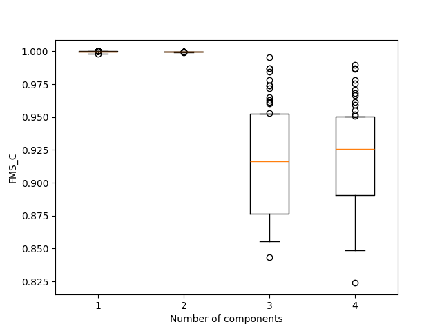
Here, we observe that over-estimating the number of components results in a loss of replicable of the patterns, indicated by low FMS.

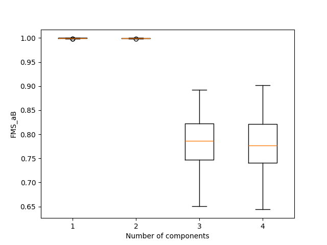
Compute and assess replicability II.

There is an alternative way to estimate the replicability of the uncovered patterns, including the factors corresponding to mode=0, and mode=1 [ErdHosCT+25]. By using only the indices present in both subsets (e.g. the factors corresponding to the subjects’ data included in both factorizations)

replicability_alt = {}
for rank in models.keys():
    replicability_alt[rank] = []
    for repeat in range(repeats):
        for i, model_i in enumerate(models[rank][repeat]):
            for j, model_j in enumerate(models[rank][repeat]):
                if i >= j:  # include every pair only once and omit i == j
                    continue
                weights_i, (aB_i, C_i) = model_i
                weights_j, (aB_j, C_j) = model_j

                indices_subset_i = sorted(split_indices[rank][repeat][i])
                indices_subset_j = sorted(split_indices[rank][repeat][j])

                common_indices = sorted(list(set(indices_subset_i).intersection(set(indices_subset_j))))
                indices2use_i = []
                indices2use_j = []

                for common_idx in common_indices:
                    indices2use_i.append(indices_subset_i.index(common_idx))
                    indices2use_j.append(indices_subset_j.index(common_idx))

                aB_i = np.concatenate([aB_i[idx] for idx in indices2use_i])
                aB_j = np.concatenate([aB_j[idx] for idx in indices2use_j])
                fms = tlviz.factor_tools.factor_match_score(
                    (weights_i, (C_i, aB_i)), (weights_j, (C_j, aB_j)), consider_weights=False
                )
                replicability_alt[rank].append(fms)

ranks = sorted(replicability_alt.keys())
data = [np.ravel(replicability_alt[r]) for r in ranks]

fig, ax = plt.subplots()
ax.boxplot(data, positions=ranks)
ax.set_xlabel("Number of components")
ax.set_ylabel("FMS_aB")
plt.show()

common_indices contains the indices (e.g. subjects/samples) present in both subsets, but since the position of each index can change (e.g. sample no 3 is not guaranteeed at the third position in all subsets as the first and second samples might be omitted) we need to utilize the indices in the original tensor input.

Similar results can be observed with this approach in terms of the replicability of the patterns.